Simulation properties

In the Model Editor window, you can left click on the Simulation Properties button. A small window will pop up where you can change various options. The displayed options depend on the type of model you use: Static or Dynamic.

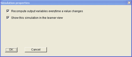
If your model is static, not having a time variable, you can check or uncheck the following options:

•

Recompute output variables every time a value changes: select this option if you want SimQuest to update the model’s output value every time the learner makes a change to one of the input variables. If unchecked, you can add an action button to your interface with the action Compute. Doing so, the learner can decide for him or herself when values should be calculated.

•	Show in learner view: if you uncheck this box, the complete level is invisible for the learner.

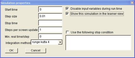
If you are using a dynamic model, so with a time variable included, you have the following options concerning Simulation Properties:

•	Steps per screen update: type the number of calculation steps between each screen update. The default value is 1, but increasing this value will significantly increase the running speed of your simulation if you have a complex model.

•	Min. real time/step: to slow down your simulation, you can increase the minimum amount of seconds that every time step should last.

•	Integration method: select the method you want to use to numerically solve the differential equations in your model:

Runge Kutta 4: the default method, recommended for most cases. The fourth order Runge Kutta method is an accurate, 4th order integration method with a variable integration step size. Only in case of a very ‘stiff’ systems of differential equations, or, in other words, systems which contain variables that change in widely varying time scales, calculation times may be very high. This is because the integration step sizes chosen by the algorithm will be very small. In these cases you may want to consider one of the other methods.

Euler: first order Euler, the least accurate, but fastest method of the four. This method uses only one function evaluation per step, and you may therefore want to consider using this method on slower computers or with more complex, but generally stable models.

Adams Bashfort 2: an integration method that uses a 2nd order Lagrange polynomial to extrapolate differential values in the past to differential values in the future, and integrate these to obtain an estimate of the next desired function value.

Runge Kutta 2: a second order integration algorithm. Use this method as a compromise between speed (Euler) and accuracy (Runge Kutta 4).

•	Disable input variables during run time: checking this box will all inputs in an interface inaccessible while the simulation is running.

•	Show in learner view: if you uncheck this box, the complete level is invisible for the learner.

A stop condition can be used to stop the simulation when one or more variables have reached specified values. For example, when you enter x => 3 in this field, the simulation will stop running whenever the value of the variable x exceeds 3. To activate the stop condition, check the box that reads ‘Use the following stop condition’. If you want to use a combination of stop conditions, you can use & (if both conditions should apply at the same time) or | if either of the two should apply.